
Introduction
Several key topics:
- The architecture and components of a Spark Application.
- The life cycle of a Spark Application inside and outside of Spark.
- Important low-level execution properties, such as pipelining.
- What it takes to run a Spark Application.
The Architecture of a Spark Application
More Information
Some of the high-level components of a Spark Application:
- The Spark driver
- The Spark executors
- The cluster manager
The Spark driver
It is the controller of the execution of a Spark Application and maintains all of the state of the Spark cluster (the state and tasks of the executors).
The Spark executors
Spark executors perform the tasks assigned by the Spark driver. Executors have one core responsibility: take the tasks assigned by the driver, run them, and report back their state (success or failure) and results. Each Spark Application has its own separate executor processes.
Number of executors in a single node
By default, each node have an executor. However, you can config single node to run multiple executors.
The cluster manager
The cluster manager is responsible for maintaining a cluster of machines that will run your Spark Application(s). A cluster manager will have its own driver (master) and worker abstractions. The core difference is that these are tied to physical machines rather than processes (as they are in Spark).
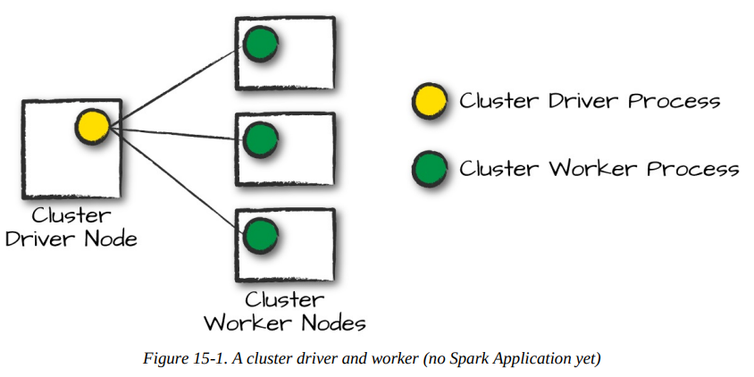
In the above illustration, on the left is the Cluster Driver Node .The circles represent daemon processes running on and managing each of the individual worker nodes.
When it comes time to actually run a Spark Application, we request resources from the cluster manager to run it. Depending on how our application is configured, this can include a place to run the Spark driver or might be just resources for the executors for our Spark Application. Over the course of Spark Application execution, the cluster manager will be responsible for managing the underlying machines that our application is running on.
Spark currently supports three cluster managers: standalone cluster manager, Apache Mesos, and Hadoop YARN.
Execution Modes
An execution mode gives you the power to determine where the aforementioned resources are physically located when you go to run your application. You have three modes to choose from:
- Cluster mode
- Client mode
- Local mode
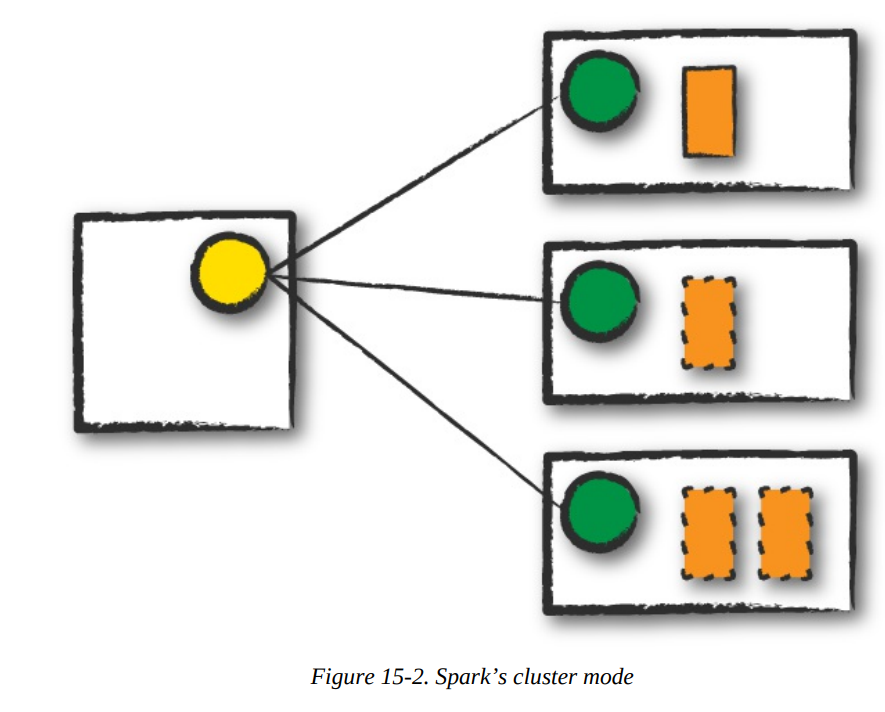
Cluster mode
In cluster mode, a user submits a pre-compiled JAR, Python script, or R script to a cluster manager.
Info
The cluster manager launches the driver process on a worker node inside the cluster, in addition to the executor processes.
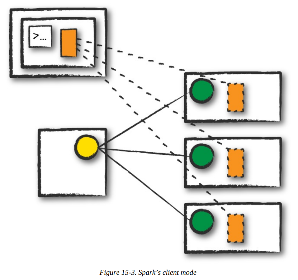
Client mode
In client mode, the Spark driver remains on the client machine that submitted the application.
Info
The client machine is responsible for maintaining the Spark driver process, and the cluster manager maintains the executor processses.
Local mode
In local mode, it runs the entire Spark Application on a single machine.
Info
It achieves parallelism through threads on that single machine.
Note
This is a common way to learn Spark, to test your applications, or experiment iteratively with local development.
The Life Cycle of a Spark Application (Outside Spark)
We assume that a cluster is already running with four nodes, a driver (not a Spark driver but cluster manager driver) and three worker nodes.
Client Request
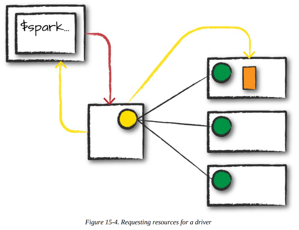
- The first step, this will be a pre-compiled JAR or library, you are executing code on your local machine and you’re going to make a request to the cluster manager driver node.
- We are explicitly asking for resources for the Spark driver process only.
- We assume that the cluster manager accepts this offer and places the driver onto a node in the cluster.
- The client process that submitted the original job exits and the application is off and running on the cluster.
./bin/spark-submit \
	--class \
	--master \
	--deploy-mode cluster \
	--conf = \
	... # other options \
	<application-jar> \
	[application-arguments]
Launch
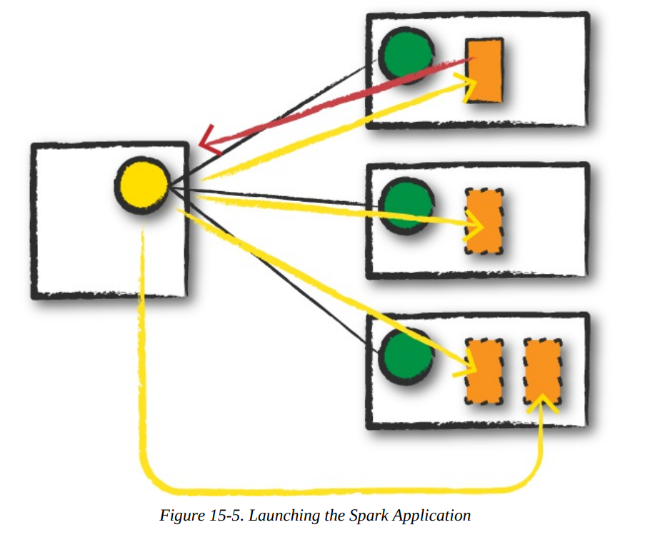
- The driver process begins running user code, which must include a
SparkSessionthat initializes a Spark cluster (e.g., driver + executors). - The
SparkSessionwill communicate with the cluster manager (the darker line), asking it to launch Spark executor processes across the cluster (the lighter lines). - The number of executors and their relevant configurations are set by the user via the command-line arguments in the original
spark-submit call. - The cluster manager responds by launching the executor processes and sends the relevant information about their locations to the driver process.
Execution
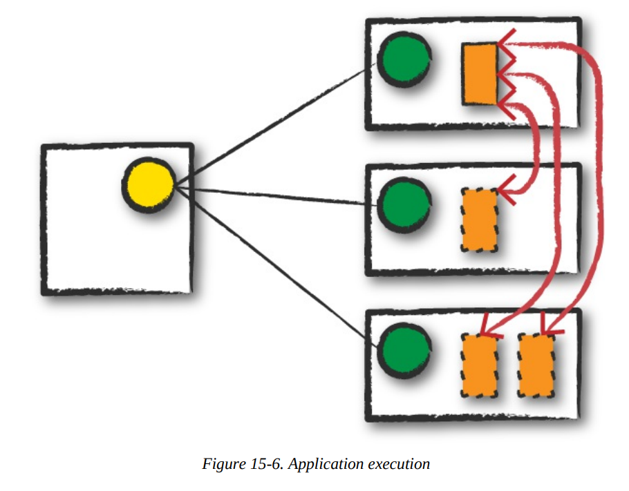
- The driver and the workers communicate among themselves, executing code and moving data around.
- The driver schedules tasks onto each worker, and each worker responds with the status of those tasks and success or failure.
More Information
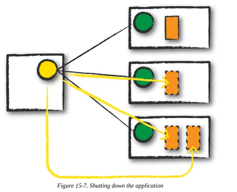
Completion
After a Spark Application completes, the driver process exits with either success or failure. The cluster manager then shuts down the executors in that Spark cluster for the driver. At this point, you can see the success or failure of the Spark Application by asking the cluster manager for this information.
The Life Cycle of a Spark Application (Inside Spark)
More information
The SparkSession
Important
The first step is always creating
SparkSession. From it, you can access all of low-level and legacy contexts and configurations.
from pyspark.sql import SparkSession

spark = SparkSession.builder.master("local").appName("Word Count")\
.config("spark.some.config.option", "some-value")\
.getOrCreate()
The SparkContext
Info
A SparkContext object within the SparkSession represents the connection to the Spark cluster. It help user communicate with some of Spark’s lower APIs.
from pyspark.context import SparkContext

sc = SparkContext.getOrCreate()
Logical Instructions
Logical instructions to physical execution
Mentioned at
To understand better, how Spark takes your code and actually runs the commands on the cluster, let’s flow this section. We are going to do a three-step job: using a simple DataFrame, we’ll repartition it, perform a value-by-value manipulation, and then aggregate some values and collect the final result.
df1 = spark.range(2, 10000000, 2)
df2 = spark.range(2, 10000000, 4)

step1 = df1.repartition(5)
step12 = df2.repartition(6)
step2 = step1.selectExpr("id * 5 as id")
step3 = step2.join(step12, ["id"])
step4 = step3.selectExpr("sum(id)")

step4.collect() # 2500000000000

step4.explain()
== Physical Plan ==
*HashAggregate(keys=[], functions=[sum(id#15L)])
+- Exchange SinglePartition
+- *HashAggregate(keys=[], functions=[partial_sum(id#15L)])
+- *Project [id#15L]
+- *SortMergeJoin [id#15L], [id#10L], Inner
:- *Sort [id#15L ASC NULLS FIRST], false, 0
: +- Exchange hashpartitioning(id#15L, 200)
: +- *Project [(id#7L * 5) AS id#15L]
: +- Exchange RoundRobinPartitioning(5)
: +- *Range (2, 10000000, step=2, splits=8)
+- *Sort [id#10L ASC NULLS FIRST], false, 0
+- Exchange hashpartitioning(id#10L, 200)
+- Exchange RoundRobinPartitioning(6)
+- *Range (2, 10000000, step=4, splits=8)
Let’s walk through the above Physical Plan The Spark plan provides a detailed breakdown of the physical execution plan:
- HashAggregate: This operator performs an aggregation, in this case, calculating the sum of the
idcolumn.- Exchange SinglePartition: This operator gathers all partitions to a single partition for the final aggregation.
- HashAggregate: This operator performs a partial aggregation on each partition.
- Project: This operator selects the
idcolumn. - SortMergeJoin: This operator joins the two DataFrames based on the
idcolumn.- Sort: Sorts each DataFrame by the join key.
- Exchange hashpartitioning: Redistributes the data based on the hash of the join key.
- Project: This operator multiplies the
idcolumn by 5. - Exchange RoundRobinPartitioning: Redistributes the data into 5 partitions.
- Range: This operator generates the initial range of numbers.
Spark range
By default when you create a DataFrame with range, it has eight partitions.
A Spark Job
In general, there should be one Spark job for one action. Actions always return results. Each job breaks down into a series of stages, the number of which depends on how many shuffle operations need to take place.
Stages
Stages
Stages in Spark represent groups of tasks that can be executed together to compute the same operation on multiple machines. Regardless of the number of partitions, that entire stage is computed in parallel. The final result aggregates those partitions individually, brings them all to a single partition before finally sending the final result to the driver.
Hint
Spark will try to pack as much work as possible (i.e., as many transformations as possible inside your job) into the same stage, , but the engine starts new stages after operations called shuffles.
Shuffle
A shuffle represents a physical repartitioning of the data.
Example
Sorting a DataFrame, or grouping data that was loaded from a file by key (which requires sending records with the same key to the same node). This type of repartitioning requires coordinating across executors to move data around. Spark starts a new stage after each shuffle, and keeps track of what order the stages must run in to compute the final result.
Set shuffle partitions
spark.conf.set("spark.sql.shuffle.partitions", 50)
Number of partitions properly
A good rule of thumb is that the number of partitions should be larger than the number of executors on your cluster, potentially by multiple factors depending on the workload. For local machine: set this value lower because local machine is unlikely to be able to execute that number of tasks in parallel.
Tasks
Task
Each task corresponds to a combination of blocks of data and a set of transformations that will run on a single executor. A task is just a unit of computation applied to a unit of data (the partition).
Example
If there is one big partition in our dataset, we will have one task. If there are 1,000 little partitions, we will have 1,000 tasks that can be executed in parallel.
Execution Details
First, spark automatically pipelines stages and tasks that can be done together.
Example
A map operation followed by another map operation.
Second, for all shuffle operations, Spark writes the data to stable storage (e.g., disk), and can reuse it across multiple jobs.
Pipelining
Spark performs as many steps as it can at one point in time before writing data to memory or disk.
Pipelining (It's the key optimization)
Pipelining occurs at and below the RDD level. Any sequence of operations that feed data directly into each other, without needing to move it across nodes, is collapsed into a single stage of tasks that do all the operations together.
Example
If you write an RDD-based program that does a map, then a filter, then another map, these will result in a single stage of tasks that immediately read each input record, pass it through the first map, pass it through the filter, and pass it through the last map function if needed. This pipelined version of the computation is much faster than writing the intermediate results to memory or disk after each step. The same kind of pipelining happens for a DataFrame or SQL computation that does a
select, filter, and select.
Shuffle Persistence
Shuffle
When Spark needs to run an operation that has to move data across nodes, such as a reduce-by-key operation, the engine can’t perform pipelining anymore, and instead it performs a cross-network shuffle.
Spark always executes shuffles by first having the “source” tasks (those sending data) write shuffle files to their local disks during their execution stage. Then, the stage that does the grouping and reduction launches and runs tasks that fetch their corresponding records from each shuffle file and performs that computation (e.g., fetches and processes the data for a specific range of keys).
The advantage of saving the shuffle files
Saving the shuffle files to disk lets Spark run this stage later in time than the source stage (e.g., if there are not enough executors to run both at the same time), and also lets the engine re-launch reduce tasks on failure without rerunning all the input tasks.
One side effect you’ll see for shuffle persistence is that running a new job over data that’s already been shuffled does not rerun the “source” side of the shuffle. Because the shuffle files were already written to disk earlier, Spark knows that it can use them to run the later stages of the job, and it need not redo the earlier ones.
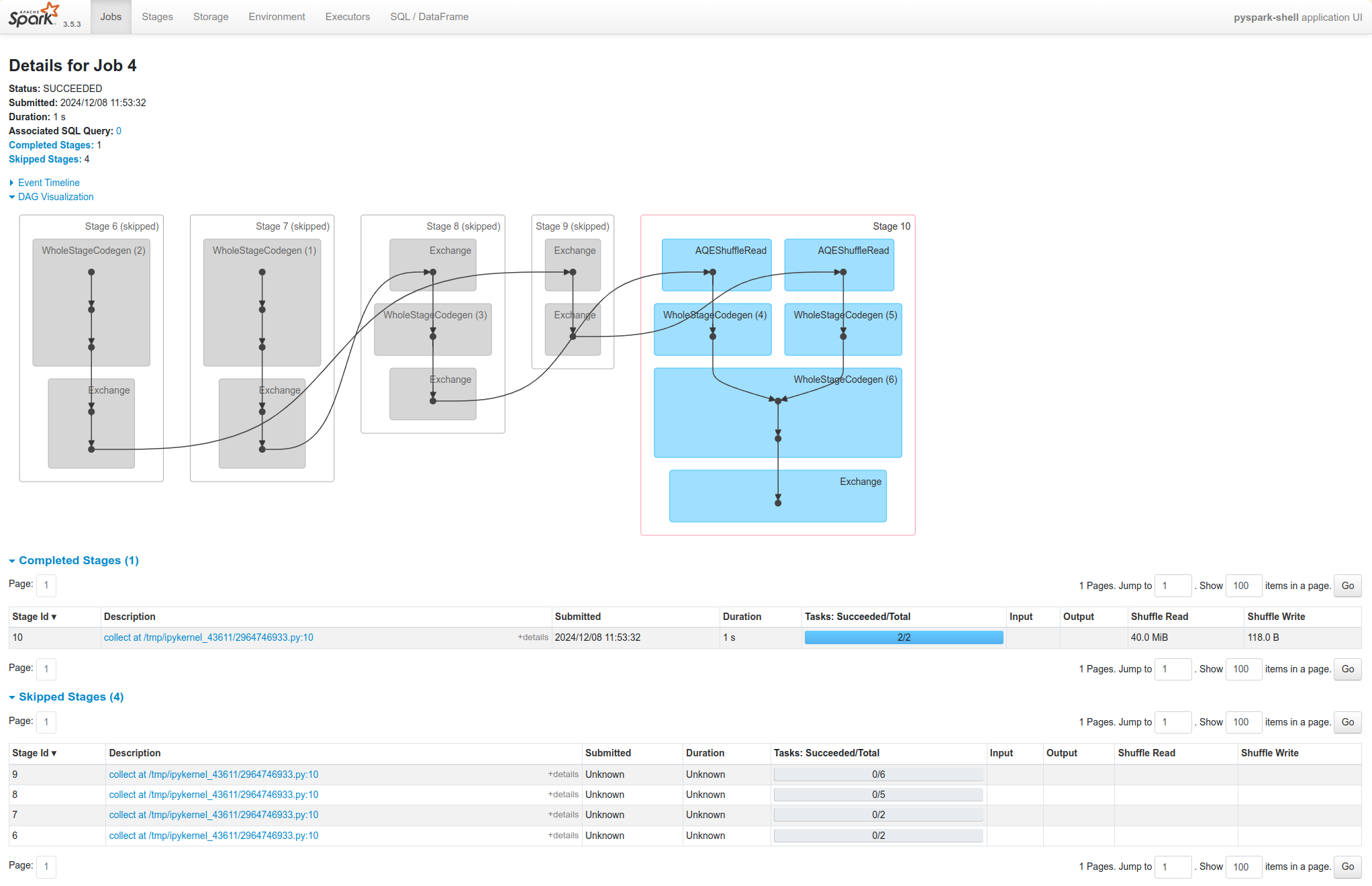
Task skipped
In the Spark UI and logs, you will see the pre-shuffle stages marked as “skipped”. This automatic optimization can save time in a workload that runs multiple jobs over the same data, but of course, for even better performance you can perform your own caching with the DataFrame or RDD cache method, which lets you control exactly which data is saved and where.
References
- Spark: The Definitive Guide by Bill Chambers and Matei Zaharia.