8. Spark SQL

Overview

Note

Spark SQL is intended to operate as an online analytic processing (OLAP) database, not an online transaction processing (OLTP) database.

How to Run Spark SQL Queries

Spark SQL CLI

./bin/spark-sql

Spark’s Programmatic SQL Interface

spark.read.json("/data/flight-data/json/2015-summary.json")\ 
.createOrReplaceTempView("some_sql_view") 
# DF => SQL 
spark.sql(""" 
	SELECT DEST_COUNTRY_NAME, sum(count) 
	FROM some_sql_view GROUP BY DEST_COUNTRY_NAME 
""")\ 
.where("DEST_COUNTRY_NAME like 'S%'")\
.where("`sum(count)` > 10")\ 
.count() # SQL => DF

SparkSQL Thrift JDBC/ODBC Server: Spark provides a Java Database Connectivity (JDBC) interface by which either you or a remote program connects to the Spark driver in order to execute Spark SQL queries. A common use case might be a for a business analyst to connect business intelligence software like Tableau to Spark.

./sbin/start-thriftserver.sh

export HIVE_SERVER2_THRIFT_PORT=<listening-port>
export HIVE_SERVER2_THRIFT_BIND_HOST=<listening-port>
./sbin/start-thriftserver.sh \ 
	--master \ 
	...

./sbin/start-thriftserver.sh \ 
	--hiveconf hive.server2.thrift.port=<listening-port> \
	--hiveconf hive.server2.thrift.bind.host=<listening-port> \ 
	--master <master-uri>
	...

You can then test this connection by running the following commands:

./bin/beeline 
beeline> !connect jdbc:hive2://localhost:10000

Catalog

The highest level abstraction in Spark SQL is the Catalog.

The Catalog

The Catalog is an abstraction for the storage of metadata about the data stored in your tables as well as other helpful things like databases, tables, functions, and views.

The catalog is available in the org.apache.spark.sql.catalog.Catalog package and contains a number of helpful functions for doing things like listing tables, databases, and functions.

Tables

Tables are logically equivalent to a DataFrame in that they are a structure of data against which you run commands.

The core difference between tables and DataFrames

You define DataFrames in the scope of a programming language, whereas you define tables within a database. This means that when you create a table (assuming you never changed the database), it will belong to the default database.

The table in Spark 2.X

Tables always contain data. There is no notion of a temporary table, only a view, which does not contain data. This is important because if you go to drop a table, you can risk losing the data when doing so.

Spark-Managed Tables

One important note is the concept of managed versus unmanaged tables. Tables store two important pieces of information. The data within the tables as well as the data about the tables; that is, the metadata. You can have Spark manage the metadata for a set of files as well as for the data.

unmanaged: define a table from files on disk.
managed: use saveAsTable on a DataFrame.

Hint

Spark also has databases, you can also see tables in a specific database by using the query show tables IN databaseName, where databaseName represents the name of the database that you want to query. If you are running on a new cluster or local mode, this should return zero results.

Creating Tables

You do not need to define a table and then load data into it; Spark lets you create one on the fly.

CREATE TABLE flights ( 
	DEST_COUNTRY_NAME STRING, 
	ORIGIN_COUNTRY_NAME STRING COMMENT "remember, the US will be most prevalent", 
	count LONG
) 
USING JSON OPTIONS (path '/data/flight-data/json/2015-summary.json')

USING AND STORED AS

The specification of the USING syntax in the previous example is of significant importance. If you do not specify the format, Spark will default to a Hive SerDe configuration. This has performance implications for future readers and writers because Hive SerDes are much slower than Spark’s native serialization. Hive users can also use the STORED AS syntax to specify that this should be a Hive table.

It is possible to create a table from a query as well:

CREATE TABLE flights_from_select USING parquet AS SELECT * FROM flights

In addition, you can specify to create a table only if it does not currently exist:

NOTE

We are creating a Hive-compatible table because we did not explicitly specify the format via USING. We can also do the following: CREATE TABLE IF NOT EXISTS flights_from_select AS SELECT * FROM flights

You can control the layout of the data by writing out a partitioned dataset

CREATE TABLE partitioned_flights USING parquet 
PARTITIONED BY (DEST_COUNTRY_NAME) 
AS SELECT DEST_COUNTRY_NAME, ORIGIN_COUNTRY_NAME, count FROM flights LIMIT 5

Creating External Tables

Example with Hive, we create an unmanaged table. Spark will manage the table’s metadata; however, the files are not managed by Spark at all. You create this table by using the CREATE EXTERNAL TABLE statement.

CREATE EXTERNAL TABLE hive_flights ( 
	DEST_COUNTRY_NAME STRING, ORIGIN_COUNTRY_NAME STRING, count LONG)
ROW FORMAT DELIMITED FIELDS TERMINATED BY ',' LOCATION '/data/flight-data-hive/'
 
-- OR
 
CREATE EXTERNAL TABLE hive_flights_2 
ROW FORMAT DELIMITED FIELDS TERMINATED BY ',' 
LOCATION '/data/flight-data-hive/' AS SELECT * FROM flights

Inserting into Tables

INSERT INTO flights_from_select 
	SELECT DEST_COUNTRY_NAME, ORIGIN_COUNTRY_NAME, count FROM flights LIMIT 20

You can optionally provide a partition specification if you want to write only into a certain partition. Note that a write will respect a partitioning scheme, as well (which may cause the above query to run quite slowly); however, it will add additional files only into the end partitions:

INSERT INTO partitioned_flights 
	PARTITION (DEST_COUNTRY_NAME="UNITED STATES") 
	SELECT count, ORIGIN_COUNTRY_NAME FROM flights 
	WHERE DEST_COUNTRY_NAME='UNITED STATES' LIMIT 12

Describing Table Metadata

DESCRIBE TABLE flights_csv
 
SHOW PARTITIONS partitioned_flights

Refreshing Table Metadata

Maintaining table metadata is an important task to ensure that you’re reading from the most recent set of data. There are two commands to refresh table metadata:

REFRESH TABLE refreshes all cached entries (essentially, files) associated with the table. If the table were previously cached, it would be cached lazily the next time it is scanned. REFRESH table partitioned_flights
REPAIR TABLE, which refreshes the partitions maintained in the catalog for that given table. This command’s focus is on collecting new partition information an example might be writing out a new partition manually and the need to repair the table accordingly: MSCK REPAIR TABLE partitioned_flights

Dropping Tables

You cannot delete tables: you can only “drop” them. You can drop a table by using the DROP keyword. If you drop a managed table (e.g., flights_csv), both the data and the table definition will be removed:

DROP TABLE flights_csv

If you try to drop a table that does not exist, you will receive an error. To only delete a table if it already exists, use DROP TABLE IF EXISTS.

DROP TABLE IF EXISTS flights_csv

Dropping unmanaged tables: If you are dropping an unmanaged table (e.g., hive_flights), no data will be removed but you will no longer be able to refer to this data by the table name.

Caching Tables

you can cache and uncache tables.

CACHE TABLE flights
 
-- OR
 
UNCACHE TABLE FLIGHTS

Views

A view specifies a set of transformations on top of an existing table. Basically just saved query plans, which can be convenient for organizing or reusing your query logic. Views can be global, set to a database, or per session.

Creating Views

To an end user, views are displayed as tables, except rather than rewriting all of the data to a new location, they simply perform a transformation on the source data at query time.

CREATE VIEW just_usa_view AS 
SELECT * FROM flights WHERE dest_country_name = 'United States'

Like tables, you can create temporary views that are available only during the current session and are not registered to a database:

CREATE TEMP VIEW just_usa_view_temp AS 
SELECT * FROM flights WHERE dest_country_name = 'United States'

Global temp views are resolved regardless of database and are viewable across the entire Spark application, but they are removed at the end of the session:

CREATE GLOBAL TEMP VIEW just_usa_global_view_temp AS 
SELECT * FROM flights WHERE dest_country_name = 'United States' 
 
SHOW TABLES

You can also specify that you would like to overwrite a view if one already exists by using the keywords REPLACE. We can overwrite both temp views and regular views:

CREATE OR REPLACE TEMP VIEW just_usa_view_temp AS 
SELECT * FROM flights WHERE dest_country_name = 'United States'

View

A view is effectively a transformation and Spark will perform it only at query time. Effectively, views are equivalent to creating a new DataFrame from an existing DataFrame.

Dropping Views

DROP VIEW IF EXISTS just_usa_view;

Databases

If you do not define one, Spark will use the default database. Any SQL statements that you run from within Spark (including DataFrame commands) execute within the context of a database. This means that if you change the database, any user-defined tables will remain in the previous database and will need to be queried differently.

WARNING

This can be a source of confusion, especially if you’re sharing the same context or session for your coworkers, so be sure to set your databases appropriately.

Creating Databases

CREATE DATABASE some_db

Setting the Database

Use the USE keyword.

USE some_db

You can query different databases by using the correct prefix:

SELECT * FROM default.flights

You can see what database you’re currently using by running the following command:

SELECT current_database()

Switch back to the default database:

USE default;

Dropping Databases

DROP DATABASE IF EXISTS some_db;

Select Statements

SELECT [ALL|DISTINCT] named_expression[, named_expression, ...] 
	FROM relation[, relation, ...] 
	[lateral_view[, lateral_view, ...]] 
	[WHERE boolean_expression] 
	[aggregation [HAVING boolean_expression]] 
	[ORDER BY sort_expressions] 
	[CLUSTER BY expressions] 
	[DISTRIBUTE BY expressions] 
	[SORT BY sort_expressions] 
	[WINDOW named_window[, WINDOW named_window, ...]] 
	[LIMIT num_rows] 
 
named_expression: 
	: expression [AS alias] 
	
relation: 
	| join_relation 
	| (table_name|query|relation) [sample] [AS alias] 
	: VALUES (expressions)[, (expressions), ...] 
		[AS (column_name[, column_name, ...])] 
		
expressions: 
	: expression[, expression, ...] 
 
sort_expressions: 
	: expression [ASC|DESC][, expression [ASC|DESC], ...]

case…when…then Statements

SELECT 
	CASE WHEN DEST_COUNTRY_NAME = 'UNITED STATES' THEN 1 
		WHEN DEST_COUNTRY_NAME = 'Egypt' THEN 0 
		ELSE -1 END 
FROM partitioned_flights

Advanced Topics

Now that we defined where data lives and how to organize it, let’s move on to querying it.

Complex Types

Structs To create one, you simply need to wrap a set of columns (or expressions) in parentheses:

CREATE VIEW IF NOT EXISTS nested_data AS 
SELECT (DEST_COUNTRY_NAME, ORIGIN_COUNTRY_NAME) as country, count FROM flights

You can even query individual columns within a struct all you need to do is use dot syntax:

SELECT country.DEST_COUNTRY_NAME, count FROM nested_data
SELECT country.*, count FROM nested_data

Lists You can use the collect_list function, which creates a list of values. You can also use the function collect_set, which creates an array without duplicate values. These are both aggregation functions and therefore can be specified only in aggregations:

SELECT 
	DEST_COUNTRY_NAME as new_name, 
	collect_list(count) as flight_counts, 
	collect_set(ORIGIN_COUNTRY_NAME) as origin_set 
FROM flights 
GROUP BY DEST_COUNTRY_NAME

Create an array manually within a column, as shown here:

SELECT DEST_COUNTRY_NAME, ARRAY(1, 2, 3) FROM flights

Query lists by position by using a Python-like array query syntax:

SELECT DEST_COUNTRY_NAME as new_name, collect_list(count)[0] 
FROM flights 
GROUP BY DEST_COUNTRY_NAME

You can also do things like convert an array back into rows. You do this by using the explode function.

CREATE OR REPLACE TEMP VIEW flights_agg AS 
	SELECT DEST_COUNTRY_NAME, collect_list(count) as collected_counts 
	FROM flights 
	GROUP BY DEST_COUNTRY_NAME
 
SELECT explode(collected_counts), DEST_COUNTRY_NAME FROM flights_agg

Functions

To see a list of functions in Spark SQL, you use the SHOW FUNCTIONS statement:

SHOW FUNCTIONS
 
SHOW SYSTEM FUNCTIONS
 
SHOW USER FUNCTIONS
 
-- Filter
SHOW FUNCTIONS "s*";
 
SHOW FUNCTIONS LIKE "collect*";

You might want to know more about specific functions themselves. To do this, use the DESCRIBE keyword, which returns the documentation for a specific function.

User-defined functions You can define functions, just as you did before, writing the function in the language of your choice and then registering it appropriately:

def power3(number:Double):Double = number * number * number 
spark.udf.register("power3", power3(_:Double):Double)

SELECT count, power3(count) FROM flights

Subqueries

In Spark, there are two fundamental subqueries. Correlated subqueries use some information from the outer scope of the query in order to supplement information in the subquery. Uncorrelated subqueries include no information from the outer scope. Each of these queries can return one (scalar subquery) or more values. Spark also includes support for predicate subqueries, which allow for filtering based on values.

Uncorrelated predicate subqueries For example, let’s take a look at a predicate subquery. In this example, this is composed of two uncorrelated queries. The first query is just to get the top five country destinations based on the data we have:

SELECT dest_country_name 
FROM flights 
GROUP BY dest_country_name 
ORDER BY sum(count) DESC 
LIMIT 5
 
+-----------------+ 
|dest_country_name|
+-----------------+ 
|    United States|
|           Canada|
|           Mexico|
|   United Kingdom|
|            Japan|
+-----------------+

Now we place this subquery inside of the filter and check to see if our origin country exists in that list:

SELECT * FROM flights 
WHERE origin_country_name IN (
	SELECT dest_country_name FROM flights 
	GROUP BY dest_country_name 
	ORDER BY sum(count) DESC 
	LIMIT 5
)

This query is uncorrelated because it does not include any information from the outer scope of the query. It’s a query that you can run on its own.

Correlated predicate subqueries Correlated predicate subqueries allow you to use information from the outer scope in your inner query. For example, if you want to see whether you have a flight that will take you back from your destination country, you could do so by checking whether there is a flight that has the destination country as an origin and a flight that had the origin country as a destination:

SELECT * FROM flights f1 
WHERE EXISTS (
	SELECT 1 FROM flights f2 
	WHERE f1.dest_country_name = f2.origin_country_name
) AND EXISTS (
	SELECT 1 FROM flights f2 
	WHERE f2.dest_country_name = f1.origin_country_name
)

Uncorrelated scalar queries You can bring in some supplemental information that you might not have previously. For example, if you wanted to include the maximum value as its own column from the entire counts dataset, you could do this:

SELECT *, (SELECT max(count) FROM flights) AS maximum FROM flights

Spark SQL Configurations

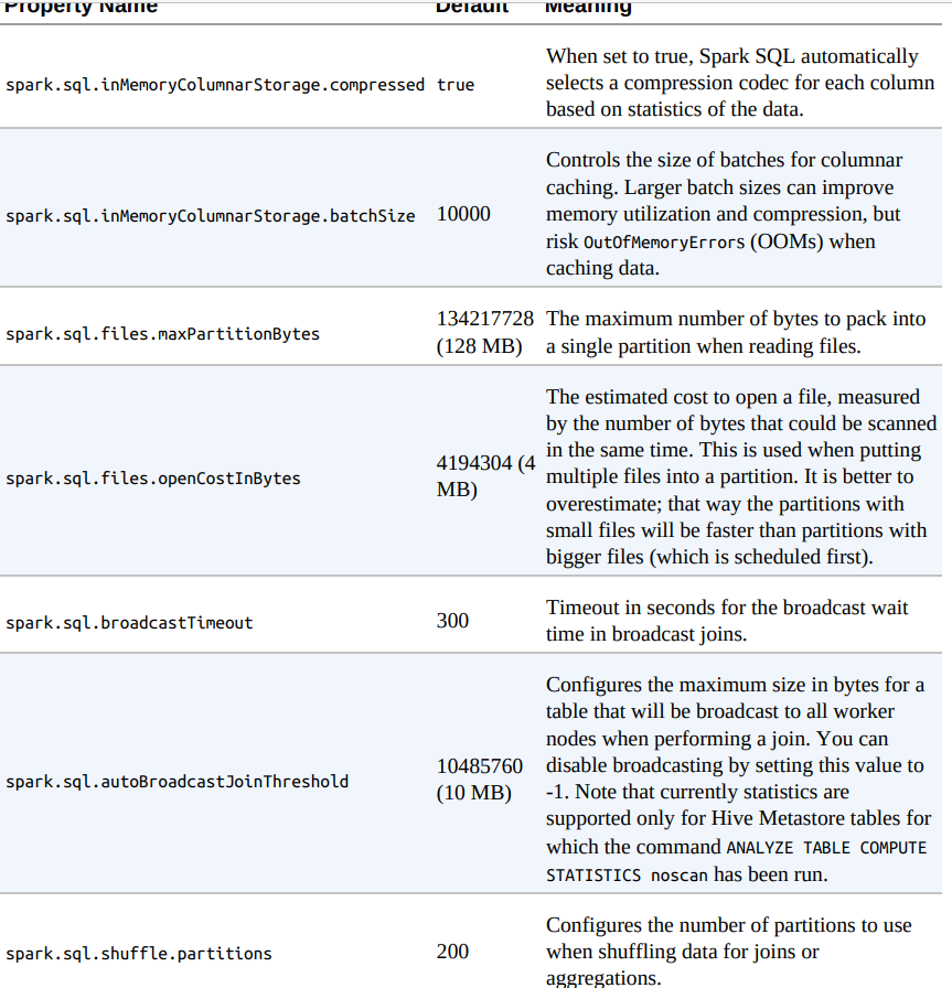
Setting Configuration Values in SQL

SET spark.sql.shuffle.partitions=20

References

Spark: The Definitive Guide by Bill Chambers and Matei Zaharia.

👩‍💻 Loi Nguyen Second Brain

Explorer

8. Spark SQL

Overview

How to Run Spark SQL Queries

Catalog

Tables

Spark-Managed Tables

Creating Tables

Creating External Tables

Inserting into Tables

Describing Table Metadata

Refreshing Table Metadata

Dropping Tables

Caching Tables

Views

Creating Views

Dropping Views

Databases

Creating Databases

Setting the Database

Dropping Databases

Select Statements

case…when…then Statements

Advanced Topics

Complex Types

Functions

Subqueries

Spark SQL Configurations

Setting Configuration Values in SQL

References

Graph View

Table of Contents