
Overview
Count operation
countis actually an action as opposed to a transformation, and so it returns immediately.
df.count()Cached DataFrame by count
You can use count to get an idea of the total size of your dataset but another common pattern is to use it to cache an entire DataFrame in memory
Aggregation Functions
count
except in this example it will perform as a transformation instead of an action.
df.select(count("StockCode")).show()count with null
There are a number of gotchas when it comes to null values and counting. For instance, when performing a count(*), Spark will count null values (including rows containing all nulls). However, when counting an individual column, Spark will not count the null values.
countDistinct
from pyspark.sql.functions import countDistinct

df.select(countDistinct("StockCode")).show() # 4070
approx_count_distinct
Often, we find ourselves working with large datasets and the exact distinct count is irrelevant. There are times when an approximation to a certain degree of accuracy will work just fine, and for that, you can use the approx_count_distinct function:
from pyspark.sql.functions import approx_count_distinct

df.select(approx_count_distinct("StockCode", 0.1)).show() # 3364
Important
approx_count_distincttook another parameter with which you can specify the maximum estimation error allowed. You will see much greater performance gains with larger datasets.
First and last
from pyspark.sql.functions import first, last

df.select(first("StockCode"), last("StockCode")).show()
min and max
from pyspark.sql.functions import min, max

df.select(min("Quantity"), max("Quantity")).show()
sum
from pyspark.sql.functions import sum

df.select(sum("Quantity")).show() # 5176450
sumDistinct
from pyspark.sql.functions import sumDistinct

df.select(sumDistinct("Quantity")).show() # 29310
avg
from pyspark.sql.functions import sum, count, avg, expr

df.select(
	count("Quantity").alias("total_transactions"),
	sum("Quantity").alias("total_purchases"),
	avg("Quantity").alias("avg_purchases"),
	expr("mean(Quantity)").alias("mean_purchases"))\
.selectExpr(
	"total_purchases/total_transactions",
	"avg_purchases",
	"mean_purchases").show()
Average with distinct
You can also average all the distinct values by specifying distinct. In fact, most aggregate functions support doing so only on distinct values.
Variance and Standard Deviation
These are both measures of the spread of the data around the mean. The variance is the average of the squared differences from the mean, and the standard deviation is the square root of the variance.
However, something to note is that Spark has both the formula for the sample standard deviation as well as the formula for the population standard deviation. These are fundamentally different statistical formulae, and we need to differentiate between them. By default, Spark performs the formula for the sample standard deviation or variance if you use the variance or stddev functions.
from pyspark.sql.functions import var_pop, stddev_pop, var_samp, stddev_samp

df.select(
	var_pop("Quantity"),
	var_samp("Quantity"),
	stddev_pop("Quantity"),
	stddev_samp("Quantity")).show()
skewness and kurtosis
Skewness measures the asymmetry of the values in your data around the mean, whereas kurtosis is a measure of the tail of data.
from pyspark.sql.functions import skewness, kurtosis

df.select(skewness("Quantity"), kurtosis("Quantity")).show()
Covariance and Correlation
Correlation measures the Pearson correlation coefficient, which is scaled between –1 and +1. Like the var function, covariance can be calculated either as the sample covariance or the population covariance. Therefore it can be important to specify which formula you want to use. Correlation has no notion of this and therefore does not have calculations for population or sample.
from pyspark.sql.functions import corr, covar_pop, covar_samp

df.select(corr("InvoiceNo", "Quantity"), covar_samp("InvoiceNo", "Quantity"), covar_pop("InvoiceNo", "Quantity")).show()
Aggregating to Complex Types
In Spark, you can perform aggregations not just of numerical values using formulas, you can also perform them on complex types.
from pyspark.sql.functions import collect_set, collect_list

df.agg(collect_set("Country"), collect_list("Country")).show()

#+--------------------+---------------------+ #|collect_set(Country)|collect_list(Country)|
#+--------------------+---------------------+
#|[Portugal, Italy,...| [United Kingdom, ...|
#+--------------------+---------------------+
Grouping
We do this grouping in two phases:
- First we specify the column(s) on which we would like to group,
- Then we specify the aggregation(s).
- The first step returns a
RelationalGroupedDataset, and the second step returns aDataFrame.
df.groupBy("InvoiceNo", "CustomerId").count().show()Grouping with expression
from pyspark.sql.functions import count

df.groupBy("InvoiceNo").agg(
	count("Quantity").alias("quan"),
	expr("count(Quantity)")).show()

#+---------+----+---------------+
#|InvoiceNo|quan|count(Quantity)|
#+---------+----+---------------+
#|   536596|   6|              6|
#...
#|  C542604|   8|              8|
#+---------+----+---------------+
Grouping with Maps
df.groupBy("InvoiceNo").agg(
	expr("avg(Quantity)"),
	expr("stddev_pop(Quantity)"))\
.show()

#+---------+------------------+--------------------+
#|InvoiceNo|     avg(Quantity)|stddev_pop(Quantity)|
#+---------+------------------+--------------------+
#|   536596|               1.5|  1.1180339887498947|
#...
#|  C542604|              -8.0|  15.173990905493518|
#+---------+------------------+--------------------+
Window Functions
You can also use window functions to carry out some unique aggregations by either computing some aggregation on a specific “window” of data, which you define by using a reference to the current data. This window specification determines which rows will be passed in to this function.
from pyspark.sql.functions import col, to_date

dfWithDate = df.withColumn("date", to_date(col("InvoiceDate"), "MM/d/yyyy H:mm"))

dfWithDate.createOrReplaceTempView("dfWithDate")
The first step to a window function is to create a window specification. Note that the partition by is unrelated to the partitioning scheme concept that we have covered thus far. It’s just a similar concept that describes how we will be breaking up our group. The ordering determines the ordering within a given partition, and, finally, the frame specification (the rowsBetween statement) states which rows will be included in the frame based on its reference to the current input row.
from pyspark.sql.window import Window
from pyspark.sql.functions import desc

windowSpec = Window\
	.partitionBy("CustomerId", "date")\
	.orderBy(desc("Quantity"))\
	.rowsBetween(Window.unboundedPreceding, Window.currentRow)
Now we want to use an aggregation function to learn more about each specific customer. An example might be establishing the maximum purchase quantity over all time. To answer this, we use the same aggregation functions that we saw earlier by passing a column name or expression. In addition, we indicate the window specification that defines to which frames of data this function will apply:
from pyspark.sql.functions import max

maxPurchaseQuantity = max(col("Quantity")).over(windowSpec)
You will notice that this returns a column (or expressions). We can now use this in a DataFrame select statement. Before doing so, though, we will create the purchase quantity rank. To do that we use the dense_rank function to determine which date had the maximum purchase quantity for every customer. We use dense_rank as opposed to rank to avoid gaps in the ranking sequence when there are tied values (or in our case, duplicate rows):
from pyspark.sql.functions import dense_rank, rank

purchaseDenseRank = dense_rank().over(windowSpec)
purchaseRank = rank().over(windowSpec)
This also returns a column that we can use in select statements. Now we can perform a select to view the calculated window values:
from pyspark.sql.functions import col

dfWithDate.where("CustomerId IS NOT NULL").orderBy("CustomerId")\
	.select(
		col("CustomerId"),
		col("date"),
		col("Quantity"),
		purchaseRank.alias("quantityRank"),
		purchaseDenseRank.alias("quantityDenseRank"),
		maxPurchaseQuantity.alias("maxPurchaseQuantity")).show()
SELECT CustomerId, date, Quantity,
rank(Quantity) OVER (
PARTITION BY CustomerId, date
ORDER BY Quantity DESC NULLS LAST
ROWS BETWEEN UNBOUNDED PRECEDING AND CURRENT ROW
) as rank,
dense_rank(Quantity) OVER (
PARTITION BY CustomerId, date
ORDER BY Quantity DESC NULLS LAST
ROWS BETWEEN UNBOUNDED PRECEDING AND CURRENT ROW
) as dRank,
max(Quantity) OVER (
PARTITION BY CustomerId, date
ORDER BY Quantity DESC NULLS LAST
ROWS BETWEEN UNBOUNDED PRECEDING AND CURRENT ROW
) as maxPurchase
FROM dfWithDate WHERE CustomerId IS NOT NULL ORDER BY CustomerId+----------+----------+--------+------------+-----------------+---------------+
|CustomerId| date|Quantity|quantityRank|quantityDenseRank|maxP...Quantity|
+----------+----------+--------+------------+-----------------+---------------+
| 12346|2011-01-18| 74215| 1| 1| 74215|
| 12346|2011-01-18| -74215| 2| 2| 74215|
| 12347|2010-12-07| 36| 1| 1| 36|
| 12347|2010-12-07| 30| 2| 2| 36|
...
| 12347|2010-12-07| 12| 4| 4| 36|
| 12347|2010-12-07| 6| 17| 5| 36|
| 12347|2010-12-07| 6| 17| 5| 36|
+----------+----------+--------+------------+-----------------+---------------+Grouping Sets
The aggregation across multiple groups. Grouping sets are a low-level tool for combining sets of aggregations together. They give you the ability to create arbitrary aggregation in their group-by statements.
dfNoNull = dfWithDate.drop()

dfNoNull.createOrReplaceTempView("dfNoNull")
SELECT CustomerId, stockCode, sum(Quantity)
FROM dfNoNull
GROUP BY customerId, stockCode
ORDER BY CustomerId DESC, stockCode DESC
/*
+----------+---------+-------------+
|CustomerId|stockCode|sum(Quantity)|
+----------+---------+-------------+
| 18287| 85173| 48|
| 18287| 85040A| 48|
| 18287| 85039B| 120|
...
| 18287| 23269| 36|
+----------+---------+-------------+
*/You can do the exact same thing by using a grouping set:
SELECT CustomerId, stockCode, sum(Quantity)
FROM dfNoNull
GROUP BY customerId, stockCode GROUPING SETS((customerId, stockCode))
ORDER BY CustomerId DESC, stockCode DESC

/*
+----------+---------+-------------+
|CustomerId|stockCode|sum(Quantity)|
+----------+---------+-------------+
|     18287|    85173|           48|
|     18287|   85040A|           48|
|     18287|   85039B|          120|
...
|     18287|    23269|           36|
+----------+---------+-------------+
*/
Working with null
Grouping sets depend on null values for aggregation levels. If you do not filter-out null values, you will get incorrect results. This applies to cubes, rollups, and grouping sets.
Simple enough, but what if you also want to include the total number of items, regardless of customer or stock code? With a conventional group-by statement, this would be impossible. But, it’s simple with grouping sets: we simply specify that we would like to aggregate at that level, as well, in our grouping set. This is, effectively, the union of several different groupings together:
SELECT CustomerId, stockCode, sum(Quantity)
FROM dfNoNull
GROUP BY customerId, stockCode GROUPING SETS((customerId, stockCode),())
ORDER BY CustomerId DESC, stockCode DESC
Note
The GROUPING SETS operator is only available in SQL. To perform the same in DataFrames, you use the rollup and cube operators—which allow us to get the same results.
Rollups
A rollup is a multidimensional aggregation that performs a variety of group-by style calculations for us. Let’s create a rollup that looks across time (with our new Date column) and space (with the Country column) and creates a new DataFrame that includes the grand total over all dates, the grand total for each date in the DataFrame, and the subtotal for each country on each date in the DataFrame:
rolledUpDF = dfNoNull.rollup("Date", "Country").agg(sum("Quantity"))\
.selectExpr("Date", "Country", "`sum(Quantity)` as total_quantity")\
.orderBy("Date")

rolledUpDF.show()

#+----------+--------------+--------------+
#|      Date|       Country|total_quantity|
#+----------+--------------+--------------+
#|      null|          null|       5176450|
#|2010-12-01|United Kingdom|         23949|
#|2010-12-01|       Germany|           117|
#|2010-12-01|        France|           449|
#...
#|2010-12-03|        France|           239|
#|2010-12-03|         Italy|           164|
#|2010-12-03|       Belgium|           528|
#+----------+--------------+--------------+
Now where you see the null values is where you’ll find the grand totals. A null in both rollup columns specifies the grand total across both of those columns:
rolledUpDF.where("Country IS NULL").show()

rolledUpDF.where("Date IS NULL").show()

#+----+-------+--------------+
#|Date|Country|total_quantity|
#+----+-------+--------------+
#|null|   null|       5176450|
#+----+-------+--------------+
Cube
A cube takes the rollup to a level deeper. Rather than treating elements hierarchically, a cube does the same thing across all dimensions. This means that it won’t just go by date over the entire time period, but also the country. To pose this as a question again, can you make a table that includes the following?
- The total across all dates and countries
- The total for each date across all countries
- The total for each country on each date
- The total for each country across all dates
from pyspark.sql.functions import sum

dfNoNull.cube("Date", "Country").agg(sum(col("Quantity")))\
.select("Date", "Country", "sum(Quantity)").orderBy("Date").show()
This is a quick and easily accessible summary of nearly all of the information in our table, and it’s a great way to create a quick summary table that others can use later on.
Grouping Metadata
Sometimes when using cubes and rollups, you want to be able to query the aggregation levels so that you can easily filter them down accordingly. We can do this by using the grouping_id, which gives us a column specifying the level of aggregation that we have in our result set. The query in the example that follows returns four distinct grouping IDs:
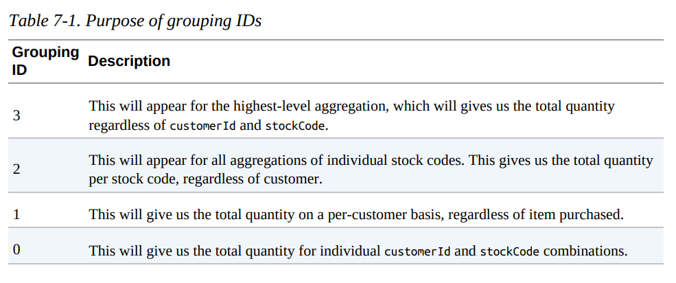
from pyspark.sql.functions import grouping_id

dfNoNull.cube("customerId", "stockCode").agg(grouping_id(), sum("Quantity")) .orderBy(expr("grouping_id()").desc) .show()

+----------+---------+-------------+-------------+
|customerId|stockCode|grouping_id()|sum(Quantity)|
+----------+---------+-------------+-------------+
|      null|     null|            3|      5176450|
|      null|    23217|            2|         1309|
|      null|   90059E|            2|           19|
...
+----------+---------+-------------+-------------+
Pivot
Pivots make it possible for you to convert a row into a column.
pivoted = dfWithDate.groupBy("date").pivot("Country").sum()For example, for USA we have the following columns: USA_sum(Quantity), USA_sum(UnitPrice), USA_sum(CustomerID). This represents one for each numeric column in our dataset (because we just performed an aggregation over all of them).
pivoted.where("date > '2011-12-05'").select("date" ,"`USA_sum(Quantity)`").show()

+----------+-----------------+
|      date|USA_sum(Quantity)|
+----------+-----------------+
|2011-12-06|             null|
|2011-12-09|             null|
|2011-12-08|             -196|
|2011-12-07|             null|
+----------+-----------------+
User-Defined Aggregation Functions
User-defined aggregation functions (UDAFs) are a way for users to define their own aggregation functions based on custom formulae or business rules. Spark maintains a single AggregationBuffer to store intermediate results for every group of input data.
To create a UDAF, you must inherit from the UserDefinedAggregateFunction base class and implement the following methods:
inputSchemarepresents input arguments as aStructTypebufferSchemarepresents intermediateUDAFresults as aStructTypedataTyperepresents the returnDataTypedeterministicis a Boolean value that specifies whether thisUDAFwill return the same result for a given inputinitializeallows you to initialize values of an aggregation bufferupdatedescribes how you should update the internal buffer based on a given rowmergedescribes how two aggregation buffers should be mergedevaluatewill generate the final result of the aggregation
The following example implements a BoolAnd, which will inform us whether all the rows (for a given column) are true; if they’re not, it will return false:
import org.apache.spark.sql.expressions.MutableAggregationBuffer
import org.apache.spark.sql.expressions.UserDefinedAggregateFunction
import org.apache.spark.sql.Row
import org.apache.spark.sql.types._

class BoolAnd extends UserDefinedAggregateFunction {
	def inputSchema: org.apache.spark.sql.types.StructType =
		StructType(StructField("value", BooleanType) :: Nil)
	def bufferSchema: StructType = StructType(
		StructField("result", BooleanType) :: Nil )
	def dataType: DataType = BooleanType
	def deterministic: Boolean = true
	def initialize(buffer: MutableAggregationBuffer): Unit = {
		buffer(0) = true
	}
	def update(buffer: MutableAggregationBuffer, input: Row): Unit = {
		buffer(0) = buffer.getAs[Boolean](0) && input.getAs[Boolean](0)
	}
	def merge(buffer1: MutableAggregationBuffer, buffer2: Row): Unit = {
		buffer1(0) = buffer1.getAs[Boolean](0) && buffer2.getAs[Boolean](0)
	}
	def evaluate(buffer: Row): Any = {
		buffer(0)
	}
}

val ba = new BoolAnd spark.udf.register("booland", ba)
import org.apache.spark.sql.functions._

spark.range(1)
	.selectExpr("explode(array(TRUE, TRUE, TRUE)) as t")
	.selectExpr("explode(array(TRUE, FALSE, TRUE)) as f", "t")
	.select(ba(col("t")), expr("booland(f)"))
	.show()

+----------+----------+
|booland(t)|booland(f)|
+----------+----------+
|      true|     false|
+----------+----------+
Pyspark with UDAFs
UDAFs are currently available only in Scala or Java. However, in Spark 2.3, you will also be able to call Scala or Java UDFs and UDAFs by registering the function.
References
- Spark: The Definitive Guide by Bill Chambers and Matei Zaharia.