Data Layer

Apache Iceberg supports several file formats, including Apache Parquet, Apache ORC, and Apache Avro. This layer contains the actual table’s data and includes data and deleted files (present if the merge-on-read mode is chosen; more on this later). The data files store the table’s records, while the delete files track rows that have been removed.
Metadata Layer
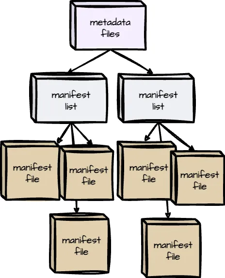
Iceberg organizes metadata as the tree architecture; the highest is the metadata files, then comes to the manifest lists, and the final is the manifest files. The metadata layer is crucial for managing large datasets and enabling key features like time travel and schema evolution.
Manifest Files
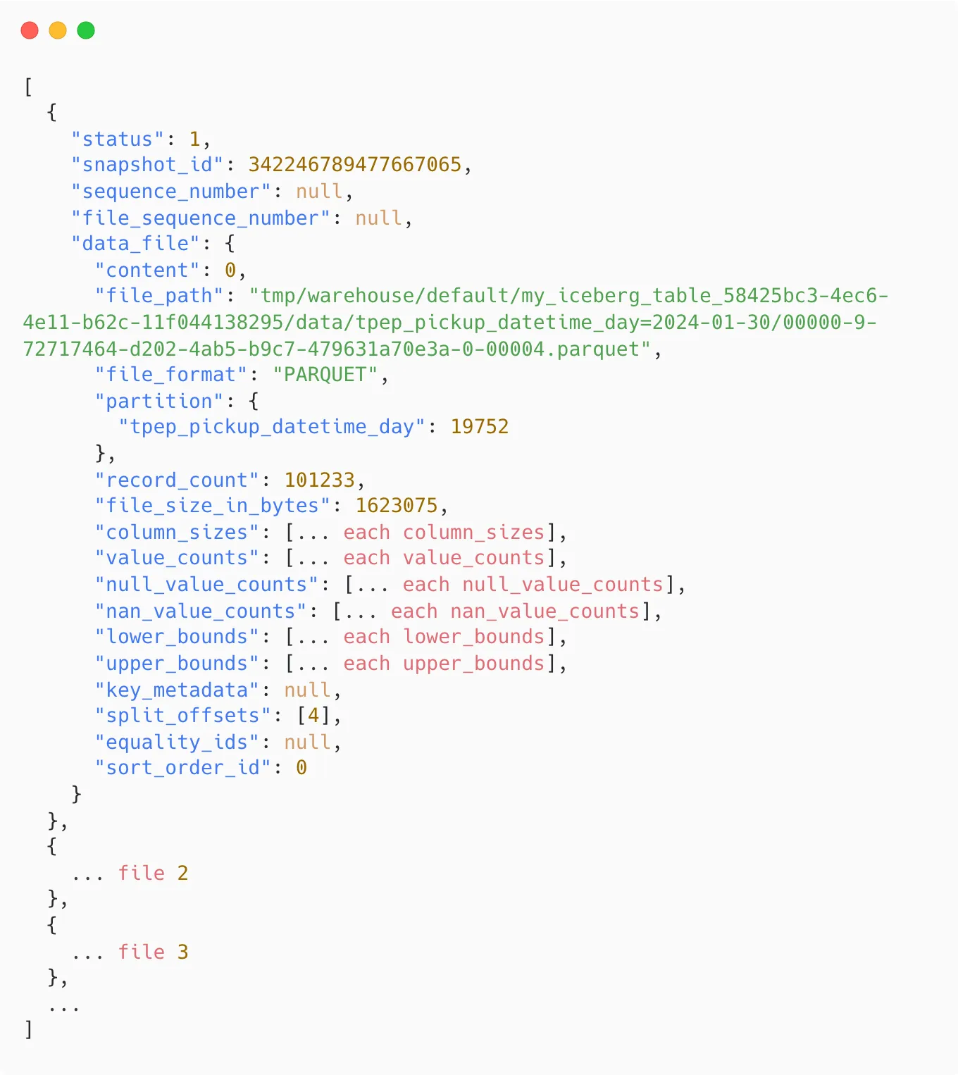 Manifest files keep track of data and delete files, as well as additional details and statistics about each file.
In the Parquet file, some of these statistics are stored in the data files themselves (min/max of each column chunk); the reader has to open each Parquet file’s footer to find the needed statistic.
However, in Iceberge, a single manifest file stores these statistics for multiple Parquet data files, which means the reader only needs to open a single file to read the statistics for all the files tracked by this manifest file. This removes the need to open many data files and improves the read performance.
Manifest Lists
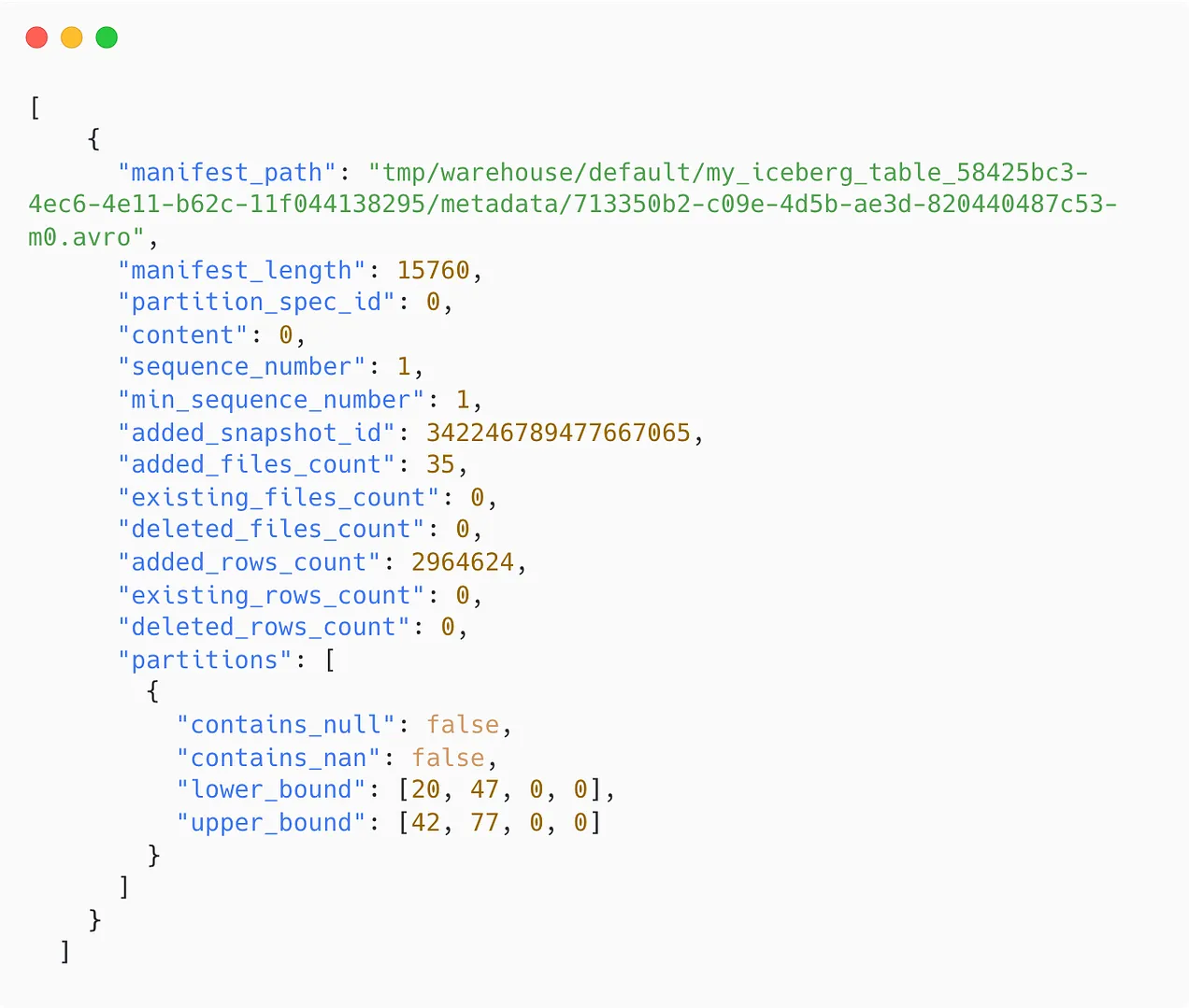
Each Iceberg table snapshot is associated with a manifest list. It contains an array of structs. Each array’s element keeps track of a single manifest file and includes information such as:
- The manifest file’s location
- The partition this manifest file belongs to
- The upper and lower bounds of the non-null partition field values are calculated across the data files tracked by this manifest file.
Metadata files
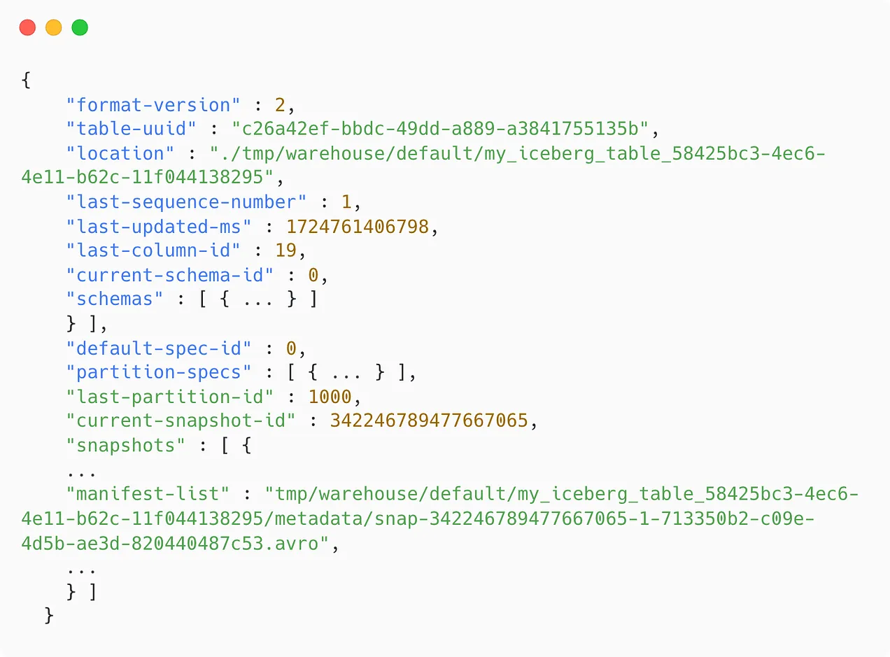
These files store the Iceberg table’s metadata at a specific time, including information such as
- The last sequence number tracks the order of snapshots in a table. This number is increased whenever the table changes.
- The table update timestamp.
- The table’s base location determines where to store data, manifests, and table metadata.
- The table’s schema
- The partition specification
- Which snapshot is the current one
- All snapshot information and its associated manifest lists.
The Catalog
All the requests must be routed through the catalog, which holds the current metadata pointer for each table. The catalog stores the location of both the current and previous metadata files, ensuring that the reader always accesses the most up-to-date information.
A critical requirement for an Iceberg catalog is supporting atomic operations when updating the metadata pointer. This ensures that all readers and writers interact with the table’s consistent state at a particular time.
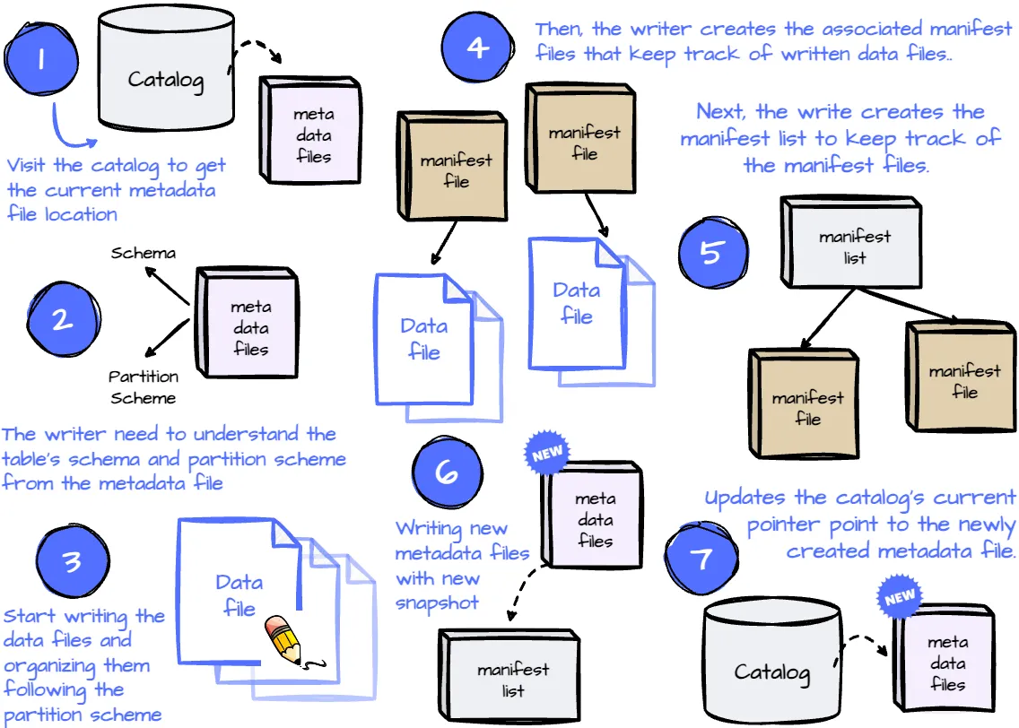
Write Operation
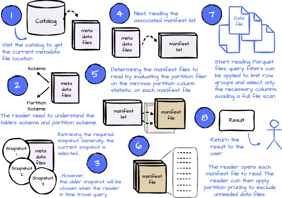
Read Operation
Compaction
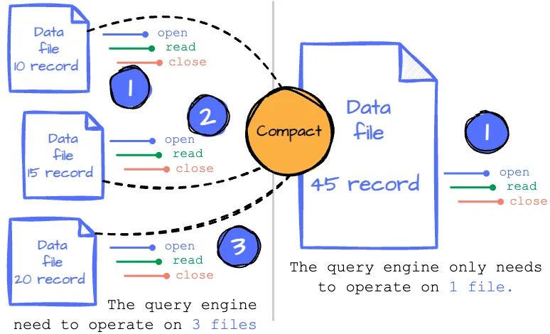
Every change in the Iceberg table results in new data files. When reading the table, after determining the necessary data files, we must open each file to read the content and close it when done. This suggests that the process becomes less efficient as the number of files we read increases.
Imagine you have an Iceberge table partitioned by the updated timestamp with day granularity. An application frequently writes to this Iceberge table daily, resulting in many data files in a single partition. You must open and close all those files when you read this partition.
What if we combine all these files into a single file so we only need to open and scan one?
In Iceberg, periodically rewriting the data in all these small files into fewer, larger files is called compaction. The writer can write as many files as they want; the compaction process will rewrite those files into larger files so they can serve the reader more efficiently. Users can control the compacting process by specifying the compaction strategy, the filter to limit which files are rewritten, the target file size, etc.
The Iceberg do not particular time to compaction data, which depend on user define manual or scheduler
Hidden Partitioning
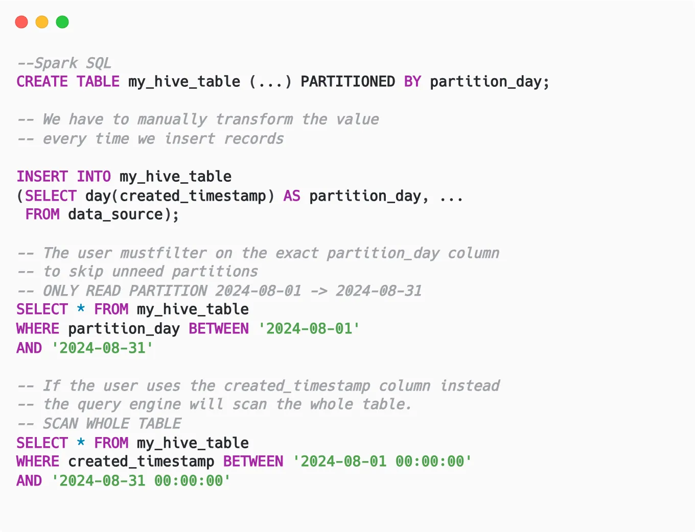
Generally, partitioning a table using transformation on a column (e.g., partition by day requires transforming the timestamp expression to day) requires creating an extra column. Users have to use this exact column to benefit from the partition pruning.
For example, a table is partitioned by day, and every record must have an extra partition_day column derived from the created_timestamp column. When users query the table, they must filter on the exact partition_day column so the query engine can only know which partitions it can skip. If the user isn’t aware of this and uses the created_timestamp column instead, the query engine will scan the whole table.
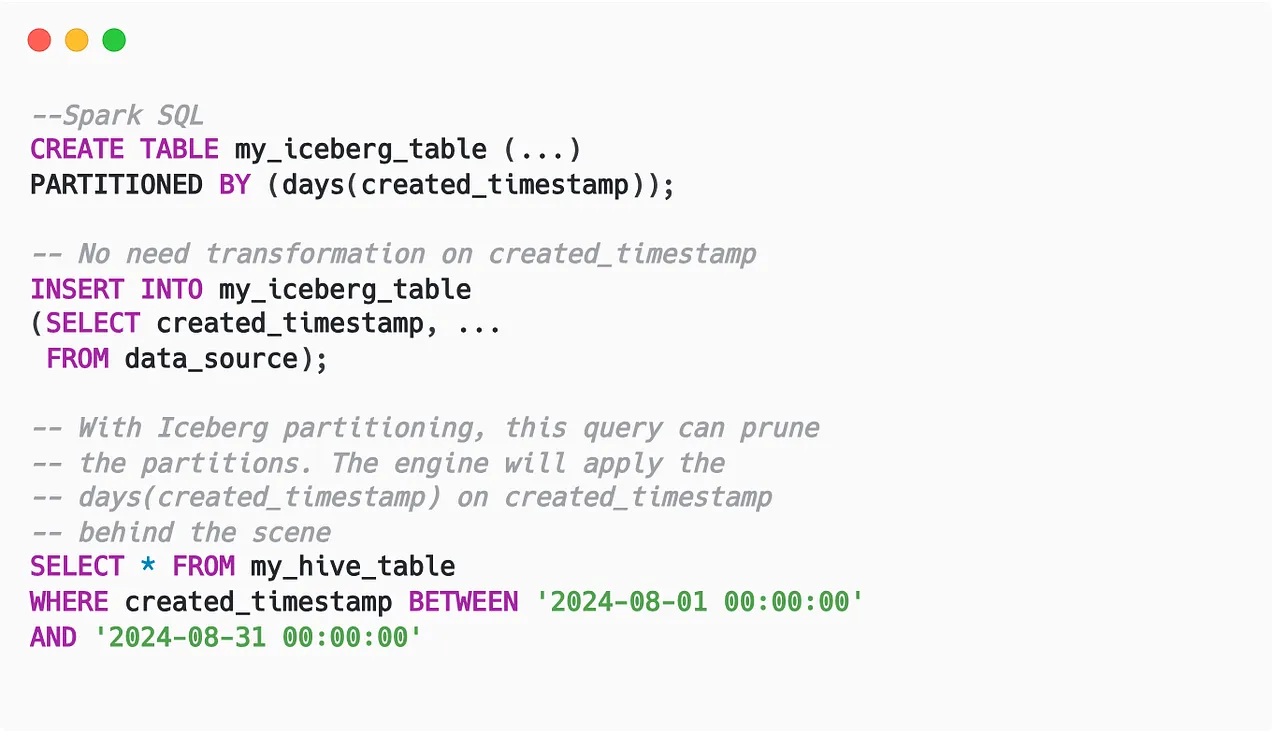
However, the latter case is more common for data analysts or business users who want to answer an analytics question; they don’t need to know about the extra column used for technical purposes (partitioning). This is where Iceberg’s hidden partitioning feature shines:
- Instead of creating additional columns to partition based on transform values, Iceberg only records the transformation used on the column.
- Thus, Iceberg stores less data in the storage because it doesn’t need to store extra columns.
- Because the metadata records the transformation on the original column, the user can filter on that column, and the query engine will apply the transformation to prune the data.
Another challenge with traditional partitioning is that it relies on the physical structure of the files being laid out into subdirectories; changing how the table was partitioned required rewriting the whole table.
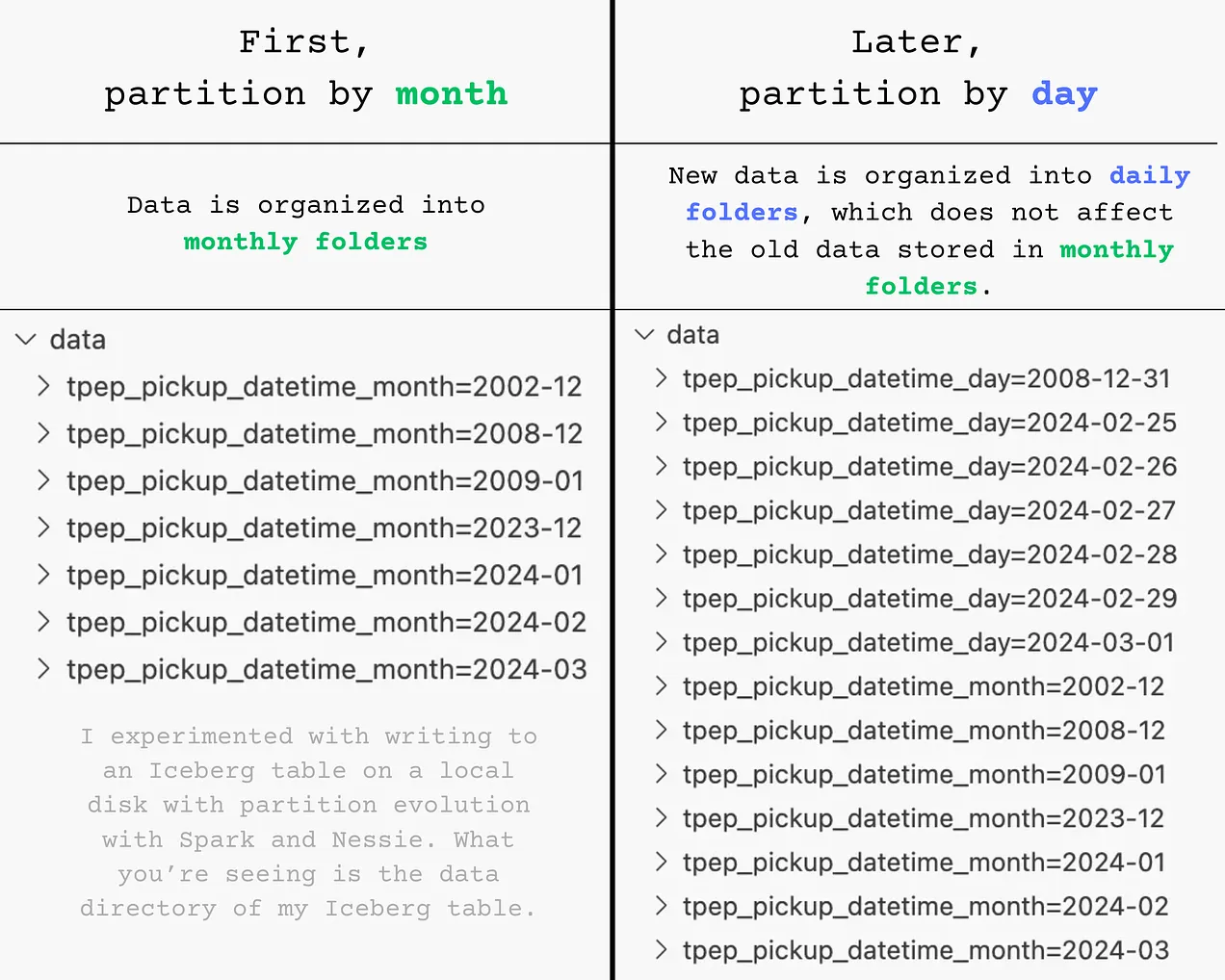
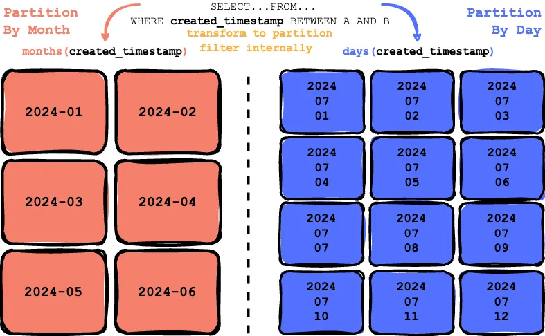
Apache Iceberg solves this problem by storing all the historical partition schemes. If the table is first partitioned by scheme A and then later partitioned by schema B, Iceberg exposes this information to the query engine to create two separate execution plans to evaluate the filter again with each partition scheme.
Given a table initially partitioned by the created_timestamp field at a monthly granularity, the transformation month(created_timestamp) is recorded as the first partitioning scheme. Later, the user updates the table to be partitioned by created_timestamp at a daily granularity, with the transformation day(created_timestamp) recorded as the second partitioning scheme.
Behind the scenes, the data is organized according to the partition scheme in place at the time of writing. For instance, the data is stored in monthly folders with month partitioning, whereas with day partitioning, it’s organized into daily folders.
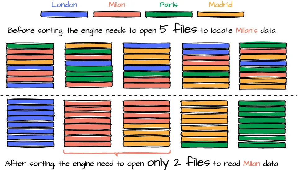
Sorting
Given an Iceberg table partitioned by day, the data contains data from four cities—London, Milan, Paris, and Madrid—the user wants to query data from Milan on 2024-08-08. After the query engine prunes unnecessary partitions, it reads the relevant data files. For the 2024-08-08 partition, there are five files in total. Since data from all four cities is scattered across these files, the engine must open all five files to locate the Milan data. However, if the data were sorted by city, with Milan’s data consolidated into two specific files, the query engine would only need to open those three files instead of all ten.
While reading data becomes more efficient with sorting, the process of writing data files may require additional effort due to the need to sort the data during writing. Moreover, to maintain global sorting across files, a compaction job is necessary to rewrite and sort the data across all files. This makes it crucial for users to carefully define the table’s sort order to leverage this optimization fully. The best practice for determining the order based on Tabular:
- Put columns most likely to be used in filters at the start of your write order, and use the lowest cardinality columns first.
- End the order with a high cardinality column, like an ID or event timestamp.
Row-level updates
When writing to storage, data files are immutable and cannot be overwritten. Any changes or updates will create new data files, which enables benefits like snapshot isolation or time travel. In Iceberg, row-level updates are handled through two modes: copy-on-write and merge-on-read.
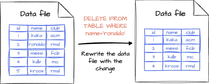
Copy-on-write (COW)
This mode is the default in Iceberg. If the table records are changed (updated or deleted), the data files associated with those records will be rewritten with the changes applied.
- Pros: Fast reading; the reader only needs to read the data without merging it with deleted or updated files.
- Cons: Slow writing; rewriting all data files will slow down updates, especially if they are too regular.
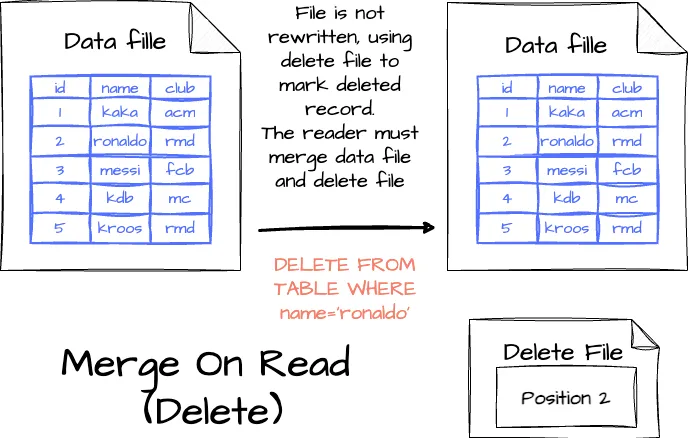
Merge-on-Read (MOR)
nstead of rewriting an entire data file, updates are made using the delete files, with changes tracked in separate files:
- Deleting a record: The record is listed in a delete file; when the reader reads the table, it will merge the data and the delete file to decide which record to skip.
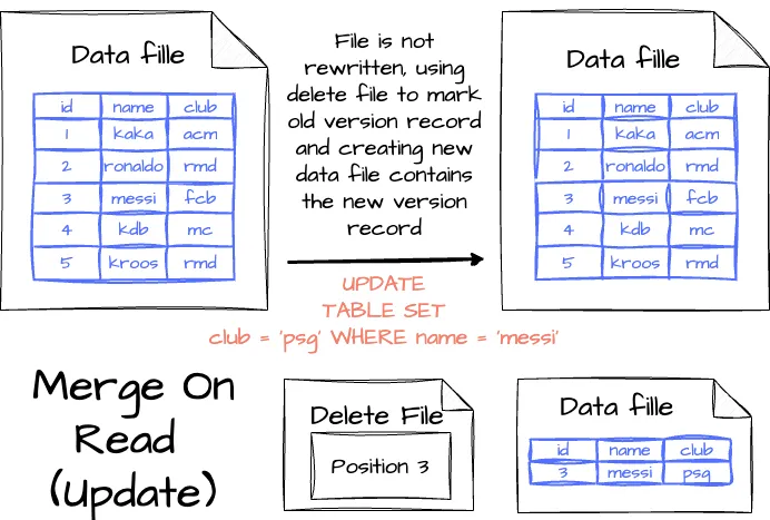
- Updating a record: The modified record is also tracked in a delete file, and then the engine creates a new data file containing the record with the updated value. When reading the table, the engine will ignore the old version of the record thanks to the deleted file and use the new version in the new data file.
With MOR mode, there will be more files in the storage than in COW mode. To minimize the data reading cost, the user can run regular compression jobs behind the scenes to reduce the number of files.
The nature of MOR is letting the reader track which records need to be ignored in the future. There are two options to control this behavior:
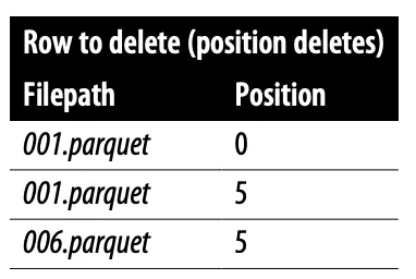
- Positional delete files: The delete file tracks rows to ignore based on their position, allowing readers to skip specific rows. While this minimizes the reading time, it increases the writing time since the writer must read the file to identify those positions.
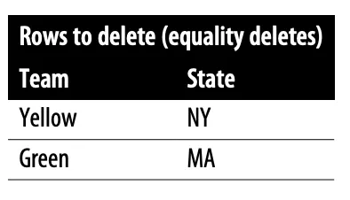
- Equality delete files: The delete files specify the deleted values; if the row has a field that matches this value, the row will be skipped. This option doesn’t require the writer to read the data file. However, it affects the reading performance because it needs to read the data file to compare each record to the deleted value.